 |
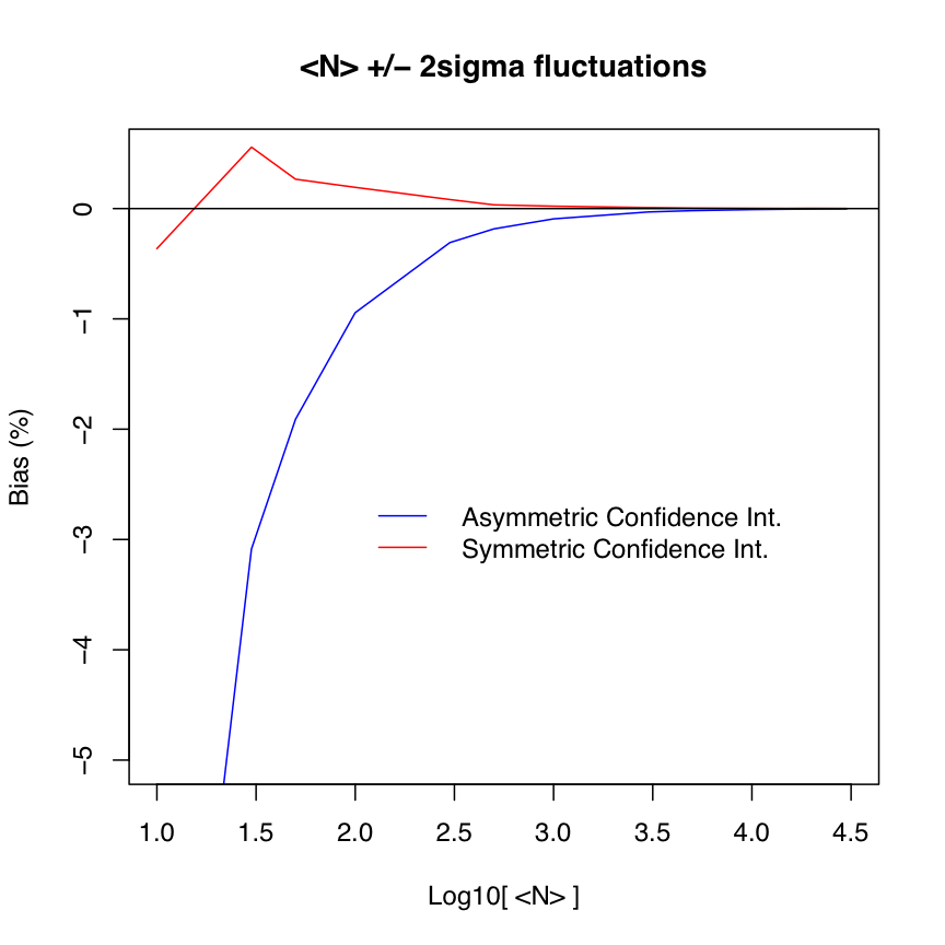
| Figure 1 - Bias (in percent) as a function of assumed input expectation value (mean count) for 2-sigma fluctuations: asymmetric (blue) and symmetric (red) confidence intervals. Click to enlarge. |
F. Masci, 4 February 2008
We have simulated the bias from inverse-variance weighted averaging of purely Poisson distributed measurements where the variances σ2i are derived from the measurements xi, i.e., σ2i = xi. Results are summarized in Tables 1 & 2 for different sigma limits and whether the confidence interval (total probability) about the assumed mean is symmetric or asymmetric.
The measurements may represent the number of photo-electrons recorded at a pixel in an imaging detector. It's important to note that the biases computed below are for pure Poisson fluctuations. Other contributions to the measurement variance such as detector read-noise, which is likely to be independent and Gaussian in nature, will dilute the bias from inverse Poisson-variance weighting. Furthermore, artificial pixel responsivity variations must be corrected before computing any inverse-variance weighted average using Poisson derived variances.
Table 1 summarizes results for the bias in the inverse Poisson-variance weighted average with the confidence interval (integrated probability) kept asymmetric about the mean μ (truth). This is due to the non-zero skewness in the Poisson distribution where the skew scales as μ-1/2. This case may be encountered when one blindly uses the same number of standard deviations about the mean for retaining data after outlier rejection, i.e., within μ ± nσ, where σ = μ1/2 for Poisson-distributed data. This ignores the possibility that the underlying distribution of the population is asymmetric, e.g., as in the Poisson regime.
We have simulated this scenario by randomly drawing 10,000,000 samples
from a Poisson distribution with assumed mean μ (column 1) and
then retaining only values xi within
μ ± 2σ and μ ± 3σ.
These values were then combined to compute an inverse Poisson-variance weighted
average (column 2):
Weighted Avg = ∑i(xi/σ2i) / ∑i(1/σ2i) = ∑i(xi/xi) / ∑i(1/xi) = Ns / ∑i(1/xi),
where Ns = sample size.
The bias in the weighted average (column 3)
is measured relative to the true mean μ:
Bias (%) = 100 * (Weighted Avg - μ) / μ.
  μ (truth)   |   Weighted Avg   |  Bias (%)  |  n in ±nσ
---------------------------------------------------------
   10             8.963957         -10.360428      2.000
   30             29.074249         -3.085837      2.000
   50             49.045239         -1.909521      2.000
   100            99.056126         -0.943874      2.000
   300            299.076390        -0.307870      2.000
   500            499.070494        -0.185901      2.000
   1000           999.063474        -0.093653      2.000
   3000           2999.059874       -0.031338      2.000
   5000           4999.058573       -0.018829      2.000
   10000          9999.108676       -0.008913      2.000
   15000          14999.109218      -0.005939      2.000
   20000          19999.021523      -0.004892      2.000
   30000          29999.093535      -0.003022      2.000
   .....................................................
   10             8.830797         -11.692025      3.000
   30             28.948477         -3.505076      3.000
   50             48.964837         -2.070327      3.000
   100            98.973086         -1.026914      3.000
   300            298.990371        -0.336543      3.000
   500            498.981064        -0.203787      3.000
   1000           998.997981        -0.100202      3.000
   3000           2998.983203       -0.033893      3.000
   5000           4998.994062       -0.020119      3.000
   10000          9998.955520       -0.010445      3.000
   15000          14998.989938      -0.006734      3.000
   20000          19999.000118      -0.004999      3.000
   30000          29999.022856      -0.003257      3.000
---------------------------------------------------------
Table 1 - Results for bias in inverse-variance weighted
          average assuming asymmetric (unbalanced)
          confidence intervals about the mean.
Table 2 summarizes results for the bias in the inverse Poisson-variance
weighted
average with the confidence interval (integrated probability) made symmetric
about the mean (truth).
This is done by first fixing an
upper threshold nU, then finding the lower
threshold nL such that:
Prob[ μ - nLσ < xi < μ ] = Prob[ μ < xi < μ + nUσ ].
10,000,000 random draws were initially made. Then only those values
xi within the new interval
μ - nLσ to μ + nUσ
were used for the weighted averaging (column 2).
All other columns are the same as defined for Table 1 above.
  μ (truth)   |   Weighted Avg   |  Bias (%)   |   nL   |   nU
-----------------------------------------------------------------
   10             9.962058         -0.379419      0.949    2.000
   30             30.165960         0.553199      1.095    2.000
   50             50.132571         0.265143      1.273    2.000
   100            100.198941        0.198941      1.400    2.000
   300            300.255111        0.085037      1.559    2.000
   500            500.158431        0.031686      1.655    2.000
   1000           1000.203027       0.020303      1.739    2.000
   3000           3000.253909       0.008464      1.826    2.000
   5000           5000.205662       0.004113      1.867    2.000
   10000          10000.167745      0.001677      1.910    2.000
   15000          15000.138307      0.000922      1.919    2.000
   20000          20000.289366      0.001447      1.923    2.000
   30000          30000.361102      0.001204      1.940    2.000
   .............................................................
   10             10.083210         0.832102      0.949    3.000
   30             30.101412         0.338040      1.278    3.000
   50             50.127484         0.254967      1.414    3.000
   100            100.137742        0.137742      1.600    3.000
   300            300.190409        0.063470      1.848    3.000
   500            500.334528        0.066906      1.923    3.000
   1000           1000.379039       0.037904      2.055    3.000
   3000           3000.423075       0.014102      2.264    3.000
   5000           5000.400008       0.008000      2.362    3.000
   10000          10000.478232      0.004782      2.460    3.000
   15000          15000.419536      0.002797      2.523    3.000
   20000          20000.534468      0.002672      2.560    3.000
   30000          30000.448127      0.001494      2.610    3.000
-----------------------------------------------------------------
Table 2 - Results for bias in inverse-variance weighted average
          assuming symmetric (balanced) confidence intervals
          about the mean.
|
|
| Figure 1 - Bias (in percent) as a function of assumed input expectation value (mean count) for 2-sigma fluctuations: asymmetric (blue) and symmetric (red) confidence intervals. Click to enlarge. |
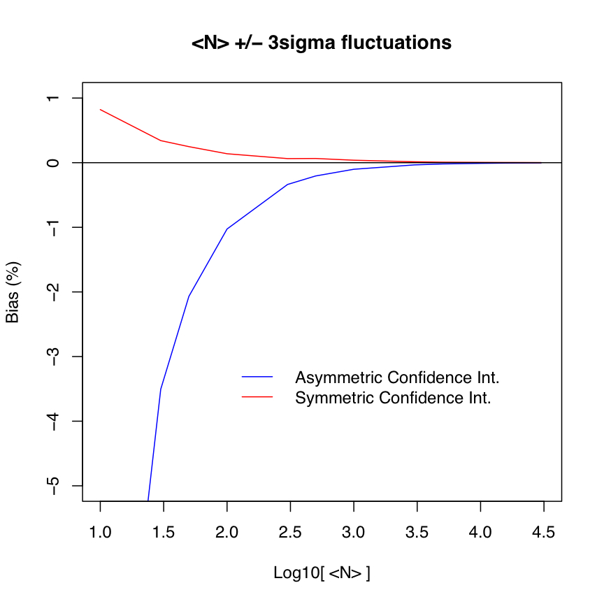 |
| Figure 2 - Bias (in percent) as a function of assumed input expectation value (mean count) for 3-sigma fluctuations: asymmetric (blue) and symmetric (red) confidence intervals. Click to enlarge. |
The above simulations were generated using the S-Plus/R Code:
PoissonBias.r